
Four years ago in May, a big story broke in Web3. UST, a stablecoin meant to always be worth one dollar, crashed to twenty cents in four days; LUNA, which backed it as collateral, slid from ninety dollars down to a fraction of a cent, wiping out eight full orders of magnitude of market cap on paper.
Plenty of institutional post-mortems of the crash exist. Most sit in the macroeconomics bucket or in on-chain mechanism analyses — herding and bank runs, that sort of thing. But we have a more interesting tool now, and I want to use it to look at how the price crash actually worked.
Mean-Field Games
Picture an exchange with a few million quant bots seated at it simultaneously, each one computing its own inventory, its counterparties, its optimal trading speed. If you honestly write down the interactions between every pair of traders, the equation system balloons into something uncomputable. It’s the same situation as the interaction among a huge number of particles in physics — you can’t model it directly with Newtonian mechanics. So we borrow the statistical-mechanics mindset: pretend each trader only cares about some averaged state of the whole crowd — say, the overall inventory distribution — and not about what any specific counterparty is doing right now. Individuals no longer face millions of hands and feet but a blurred mean field. They each make an optimal decision against the mean field, and every decision in turn contributes back to it. That’s a mean-field game.
In the algorithmic-stablecoin setting, the peg is approximately the outcome of collective equilibrium. Suppose UST drops to 0.99 on some exchange; any arbitrageur can redeem it for one dollar’s worth of LUNA and sell the LUNA, capturing the spread. As long as there’s enough of this arbitrage, fast enough, the market mechanism pulls price back to one dollar. So the firmness of the peg is the stability of the Nash equilibrium of this game.
We can model an algorithmic stablecoin this way: an individual arbitrageur’s state is his current net stablecoin position , which can sit a little off zero or very far off; the control variable is his trading speed , i.e. how much UST he swaps in or out per second. The market price is driven by the whole arbitrageur crowd’s net order flow, plus exogenous random noise:
Here is the average trading speed across the whole arbitrageur crowd, is the exogenous market noise, and measures the permanent impact of order flow on the mid price. Each arbitrageur, over the finite horizon , minimizes his own trading cost, written as a functional:
The first term is slippage friction — the faster you trade, the worse you get filled. It captures on-chain gas, exchange fees, and the immediate cost of eating through the book.
The second term is inventory risk — the further your position sits from zero, the larger the penalty for holding a de-peg-risk asset. The penalty reflects the fact that fast arbitrage lets rational traders cut their losses, while irrational participants are the ones absorbing the expected loss.
The third term is the reflexivity cost — the arbitrage itself pushes price.
Once the player count goes to infinity, this optimization problem can be written as a Hamilton–Jacobi–Bellman equation. Its main ingredient is the value function , which you can read as the total cost you expect to incur if, starting from time with inventory , you follow the optimal policy all the way to horizon . This function tells any given trader how fast to trade right now.
Since the terminal situation at is known — for instance, zeroing out inventory costs nothing, while leaving inventory incurs a penalty — the value function has a boundary condition . Roll that boundary condition back by one step: at each state you pick the optimal and read off the cost it incurs; stepping backward all the way gives you the starting strategy. This is essentially the dynamic-programming principle you’d recognize from computer science: no matter how you got to the current state, the remaining path must still be optimal. The at the tail of the equation just picks the best speed at each point. Take the derivative with respect to inside the , set it to zero, and you get a clean closed form:
The optimal trading speed equals the gradient of the value function along inventory plus the current price level, added and scaled by the reciprocal of the slippage cost. It tells the trader: where inventory makes the cost function steep, trim the position; where price has spiked into uncomfortable territory, brace against slippage.
The HJB form traces back to nineteenth-century analytical mechanics, where the principle of least action says a particle moving from A to B takes the path that minimizes the action integral among all possible paths. That same idea lets us derive things like the brachistochrone in the physical world.
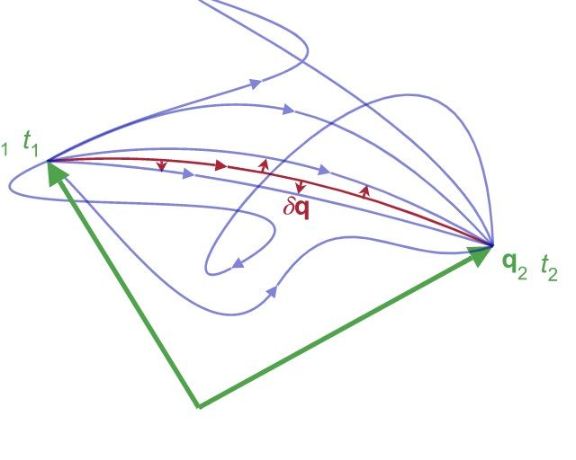
In control theory, Bellman proposed the dynamic-programming principle: the tail of an optimal policy must itself be optimal. If the fastest route from home to school goes through a particular corner store, then the segment from the store to school must itself be the fastest route from that store. Otherwise you could swap in a faster segment and shorten the total route, contradicting the assumption. Finding optimal paths, then, lends itself to the least-action principle, and in continuous time Bellman’s dynamic programming links up with the Hamilton–Jacobi equation.
The other equation is the Fokker–Planck equation. Its protagonist is the crowd-level probability density of inventory , describing what fraction of the market currently sits at each inventory level:
In physics, the Fokker–Planck equation mostly describes the statistics of diffusion. In school we all learned about Brownian motion — the random motion of a single particle. With a huge population of particles, tracking each one’s random motion is impossible and unnecessary; in the statistical-mechanics framework, we care instead about how particles distribute across space. Here we can read it as:
The inventory distribution of all traders at is known, the initial position. Every trader acts according to the coming out of the Bellman equation; simultaneously, every trader is perturbed by random noise, which is the diffusion term . Integrating the Fokker–Planck equation forward tick by tick gives the trader-inventory distribution at any future time.
The in the Bellman equation depends on the crowd’s current distribution , because price is driven by aggregate net order flow. Meanwhile the in the FP equation comes entirely from the solved in Bellman. One equation runs backward from the endpoint and needs to know the crowd distribution at every moment; the other runs forward from the start and needs the optimal policy at every moment. They’re mirror images and have to be solved together to be self-consistent.
The fixed point of this closed loop is the mean-field Nash equilibrium. At equilibrium, the stablecoin ecosystem is held at its minimum-energy point.
Renormalization Group and the Ginzburg–Landau Functional
But mean-field games are valid at one time granularity at a time. The equilibrium solved on minute bars describes the equilibrium of minute-level trader behavior; the one solved on hourly bars is hourly. When the market is calm, solutions at these two scales are compatible — the hourly equilibrium is just a simple statistical average of the minute equilibrium, differing only in resolution.
Once herding kicks in, that compatibility breaks. An arbitrageur’s current decision now depends not only on the price level but also on what the other arbitrageurs are doing. With person-to-person transmission, micro-level coordination begins spreading outward in time and space, and equilibria at different time resolutions drift apart. The renormalization group’s job here is to catch that misalignment and use it to read the market’s stability.
Working directly with the mean-field equations for RG is awkward. After a simple nonlinear transformation, the collective behavior of the whole market can be wrapped into a Ginzburg–Landau functional.
The Ginzburg–Landau functional comes from the Soviet physicist Landau’s work. Studying such different phenomena as iron becoming a magnet, water becoming ice, and a metal becoming a superconductor, Landau noticed that while the microscopic mechanisms are entirely different, near the critical point the effective free energies have strikingly similar form. Landau proposed a common approximation: near the transition, the system’s free energy can be expanded as a power series in a single variable , which mostly measures the macroscopic degree of order and is therefore called the order parameter. The order parameter distinguishes two phases — nonzero in the ordered phase, zero in the high-symmetry disordered phase. If the system itself is symmetric under , the odd-power terms must vanish, leaving the simplest form
Its interest centers on the control parameter . Take the ferromagnet as an example:
When the potential is a single-well parabola with its minimum at , corresponding to the disordered phase at high temperature — for a ferromagnet, spin orientations random and no magnetization.
When the potential becomes two symmetric valleys flanking a small bump at the center; the minima are squeezed out to , corresponding to the ordered phase at low temperature — all spins aligned in one direction, the iron block spontaneously magnetizing.
Going from high to low temperature, crosses from positive through zero to negative, and the whole system evolves from single-well to double-well.
In 1950, Landau and his student Ginzburg pushed the theory one step further. They realized that in real transitions the order parameter isn’t a single number but a spatial field , meaning the transition can progress at different rates in different places. Ginzburg added a spatial-gradient term on top of the potential to penalize neighboring sites from taking drastically different values, which encourages the system to form large regions of the same phase.
In a financial market we can locate the corresponding Ginzburg–Landau functional, which represents the market’s free energy:
The order parameter can be read as the market’s long/short tilt. means symmetric buying and selling with healthy liquidity; skewing positive or negative means the market has tilted overall to longs or shorts.
The parameter is like the market’s temperature, measuring how far the system is from criticality; measures the strength of herding.
The renormalization group was originally about scale problems in physics. Strip away small-scale detail layer by layer — coarse-graining — and track how the parameters flow during that process. If the flow equations converge to a fixed point, the state at that point is preserved under coarse-graining and is called scale-invariant.
Doing the coarse-graining along scales gives us the flow equations for and as a function of scale :
This ODE pair has two key fixed points. One is the Gaussian fixed point, , , corresponding to the normal day-to-day market.
The other is the Wilson–Fisher fixed point, , , corresponding to a system pushed past criticality by herding.
Near this fixed point, the potential goes from a symmetric parabolic bowl to an inverted Mexican hat; the market must slide to one side and a phase transition happens.
Near the critical fixed point, price jumps no longer follow a Gaussian distribution but a power law:
means you’re standing right on the critical point.
Data Validation
We can validate the theory above against data.
We use Binance one-minute candles for LUNAUSDT and USTUSDT from April to May 2022.
The whole period splits into four regimes. April 1 to May 6 is the baseline. May 7–8 is the precursor, during which Anchor Protocol saw billions of dollars of UST redemptions two days in a row. May 9–10 is the critical period, when UST first hard-de-pegged below 0.9. May 11–12 is the crash, when LUNA was minted without limit and the price was diluted to zero.
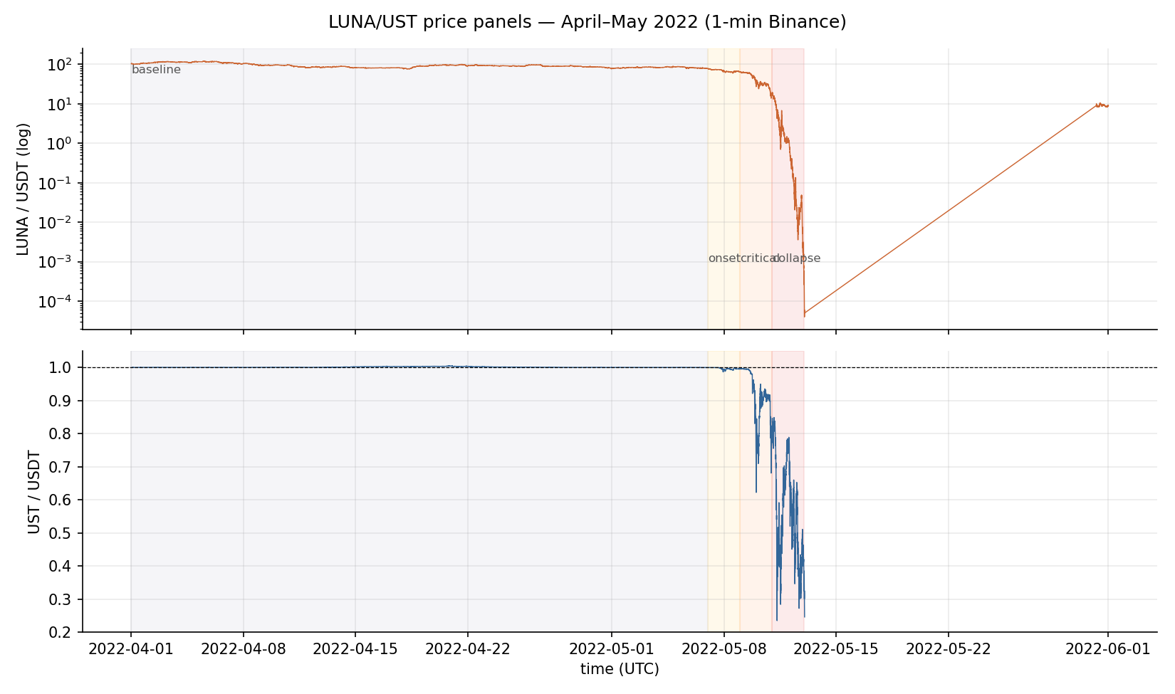
Price trajectories of LUNA and UST, April to May
The vertical axis is log-scale. You can see LUNA and UST both end up collapsing to almost nothing.
1. Baseline State Analysis
For each of the four regimes we compute the excess kurtosis and Jarque–Bera statistic (a normality test) of one-minute log returns.
UST’s baseline excess kurtosis is , with a Jarque–Bera -value of — statistically we can’t reject normality. This is consistent with the mean-field equilibrium state.
LUNA’s baseline excess kurtosis is 5.46, retaining the mild fat tail typical of crypto assets, not abnormal, and within the neighborhood of the Gaussian fixed point.
Within a single day in the precursor, UST’s one-minute kurtosis jumps from to — a 2000× leap. LUNA’s kurtosis also jumps from 5 to above 20.
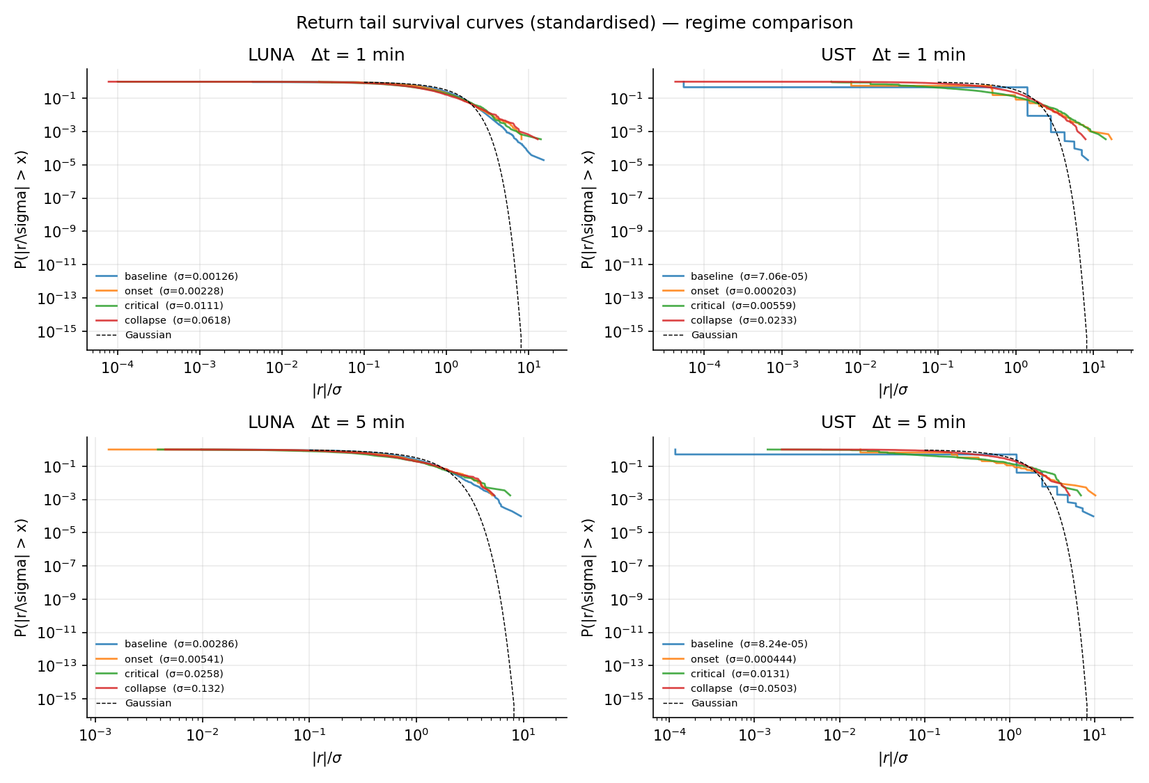
Tail survival function of standardized returns, measuring the heaviness of the tail.
These four plots put the standardized return tails for all four regimes side by side. The baseline curve hugs the black dashed line, the Gaussian reference; the other three curves diverge from Gaussian more and more as we move toward the crash. A curve that deviates from Gaussian and goes near-linear on log–log is exactly the signature of a power-law distribution.
2. Measuring the Tail Exponent
We use two methods to estimate the tail exponent: the Hill estimator and maximum likelihood. The Hill estimator is a classical tool: take the top observations, divide each by the -th largest and take the log, average, then take the reciprocal — that’s an estimate of .
Maximum likelihood assumes the data above some threshold follow a power law, writes out the likelihood function, and maximizes it.
The numbers differ slightly between the two methods, but the trends are identical.
| Asset | Baseline | Precursor | Critical | Wipeout |
|---|---|---|---|---|
| UST | 3.54 | 2.38 | 2.05 ± 0.19 | 2.94 |
| LUNA | 3.61 | 3.10 | 2.79 | 2.48 ± 0.21 |
UST’s tail exponent in the two critical days falls to 2.05, right at the lower bound of the theoretical band . LUNA in its wipeout days falls to 2.48, also comfortably inside the band. Laid out on the timeline, both trajectories flow toward the lower edge — exactly where the Wilson–Fisher fixed point sits in the RG picture.
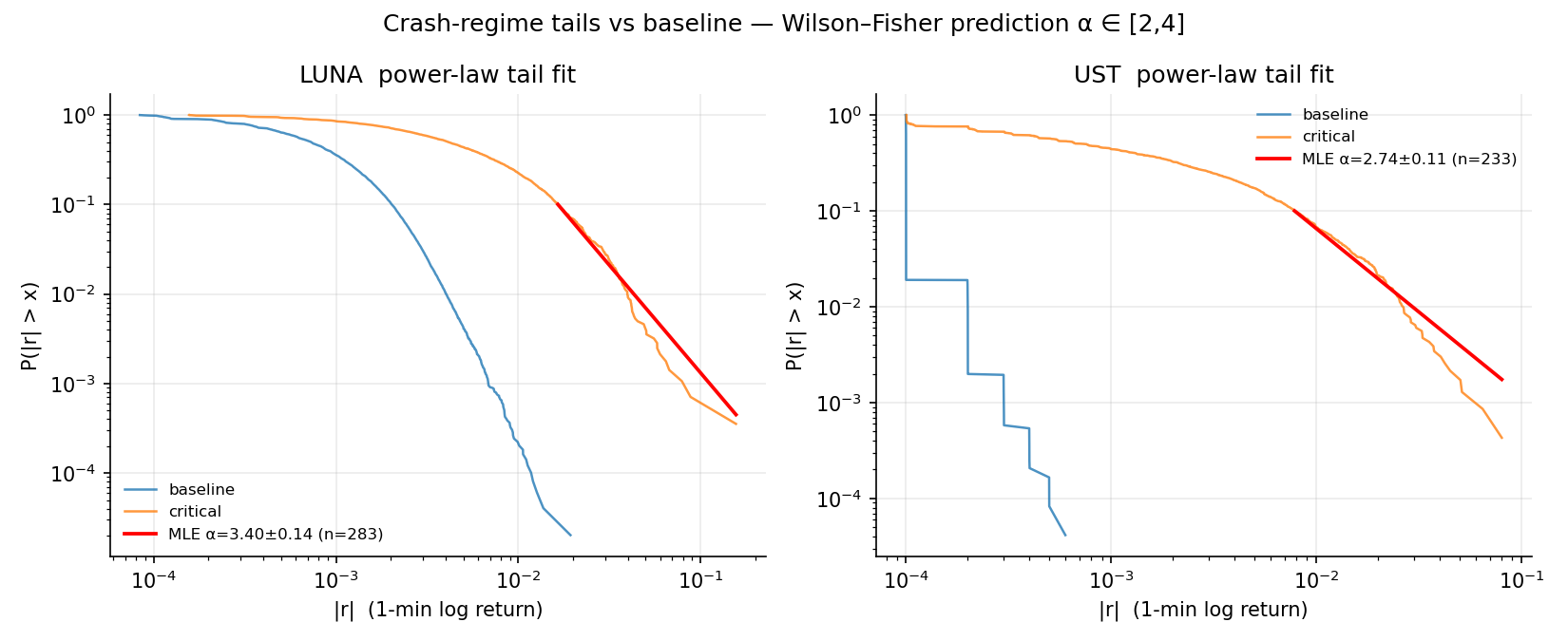
Power-law fit of the tail during the critical period
In the two plots, orange is the empirical tail survival curve during the critical period, red is the maximum-likelihood power-law fit.
3. Reading the Symmetry-Breaking Potential Well
Every trade on an exchange has two sides — one resting on the book, the maker, and one eating the resting order for immediate execution, the taker.
Total volume itself is direction-blind, because every trade has both a buyer and a seller. But the taker side isn’t direction-blind: if a trade is a buyer eating a sell order, someone was urgent enough to pay the ask, and the volume counts as taker-buy; if a seller hits a bid, someone was urgent enough to accept the bid, and the volume counts as taker-sell.
The taker is the party genuinely trying to push price at that moment; the maker is passively supplying liquidity. In the mean-field price equation , what drives price is the net speed of aggregated takers, not the total two-sided volume. Takers can be long or short.
So subtract taker-sell volume from taker-buy volume, normalize by their sum, and what you get is a proxy for the price-drift speed and the order parameter :
This quantity sits between and . Zero means balanced, positive means longs dominating, negative the reverse. Take the negative log density of ‘s distribution in each regime and the resulting curve is the empirical effective potential .
That said, as an algorithmic stablecoin, UST’s deepest sell pressure really comes from Terra’s on-chain redemption mechanism, and that flow doesn’t pass through Binance’s order book. So this data is only a local slice of the story.
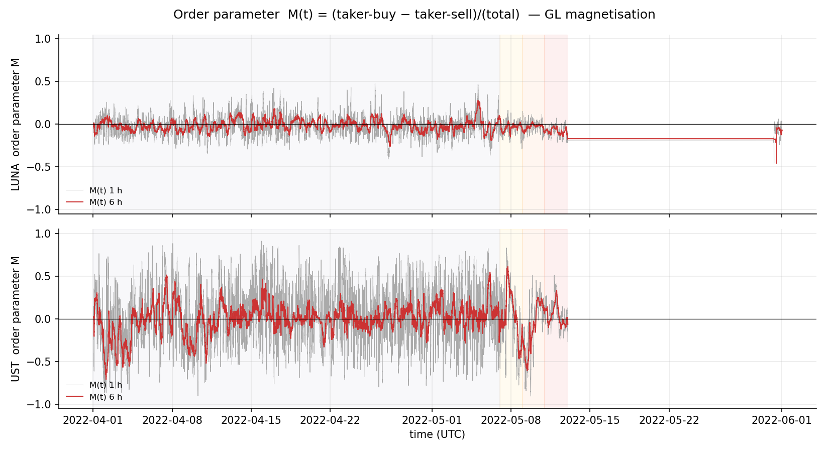
Order parameter M(t) as a time series

Shape of the empirical potential well across the four regimes
For UST, the baseline well is a single-bottom parabola with its base glued tightly to and steep walls — the case of the Ginzburg–Landau functional.
In the precursor the parabola flattens out; begins drifting toward zero.
In the critical period the well becomes flat-bottomed with shoulders, showing an obvious asymmetric structure; the central minimum no longer monopolizes the valley, and a new candidate well bulges out on the left.
In the wipeout period, you can see the central spot lifted outright and probability mass shifted almost entirely to the non-zero flanks — especially the negative side.
Single-well bowl, flat-bottomed with shoulders, raised center with twin valleys: these three steps map almost perfectly to the three schematic panels in the theory as goes from positive, through zero, to negative. An inverted Mexican hat, from top to bottom, grown right out of the data.
4. Flow of the Hurst Exponent Across Fixed Points
The Hurst exponent measures price memory — whether today’s move is statistically correlated with yesterday’s and the day before’s. Detrended fluctuation analysis gives a rolling via
is standard random walk, i.e. the Gaussian fixed point. means trending — a rise is more likely to keep rising. means mean-reverting — a rise is more likely to get pulled back.
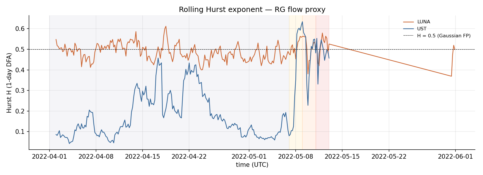
Hurst exponent on a one-day rolling window
LUNA’s baseline wanders around 0.47, consistent with the theoretical prediction — a Brownian motion.
UST’s baseline is slightly lower, hovering between 0.1 and 0.2.
In the critical period, UST’s rockets from around 0.15 to near 0.6 in under a day, vaulting a full 0.45. The system crosses the watershed at , and de-pegs. LUNA over the same window climbs from 0.47 to 0.58, also stepping across the de-peg threshold.
You can also notice that in April and early May, UST was already showing early signs of drifting off the baseline fixed point. Combined with the fundamental events of the time, we can read out some causal links:
The first episode, late April 13 to April 15, where surged to 0.336, coincides with Anchor Protocol’s deposit growth slowing obviously and net inflows turning negative. The market probably began collectively questioning whether that 19.5% headline yield was itself sustainable.
The second, April 16–17, where was pulled all the way up to the precursor-window high of 0.457, overlaps tightly with Terra’s public discussion of the 4pool architecture heating up.
The 4pool architecture refers to migrating UST’s Curve liquidity from 3pool to a new pool composed of UST, FRAX, USDC, and USDT. But that meant the arbitrage liquidity that repairs de-pegs would temporarily thin out, weakening the market’s spring.
The third, April 21–23, saw holding between 0.38 and 0.434 for three consecutive days without retreat. These three days are precisely when 4pool went live on the Fantom network, right during the event where UST liquidity was being pulled from Curve 3pool and migrated to the new pool.
A Vision for the Stablecoin Ecosystem
LUNA/UST’s collapse meant that pure algorithmic designs relying solely on the mint-and-burn of volatile assets to maintain the peg largely exited the stage. The baton passed to centralized stablecoins backed one-for-one by real fiat and short-term Treasuries, like USDT, USDC, and PYUSD; to DAI/USDS, which starts from overcollateralized crypto and gradually introduces on-chain Treasuries as ballast; and to synthetic dollars supported by perpetuals funding-rate arbitrage, like USDe.
The synthetic-dollar camp is the most worth discussing, because it’s the only surviving design whose base logic is still algorithmic in the post-UST world.
USDe uses short perpetuals on centralized exchanges to hedge spot longs and earns funding rate as yield.
As long as the perpetuals market sits in a positive funding structure where longs pay shorts, this hedge pays for itself. But the funding rate is a quantity that changes sign. Once the market enters a persistent shorts-dominant structure, funding flips from positive to negative; what used to be income becomes expense, and the hedge starts eating into the system’s structure. That is, in practice, a form of de-peg. Indeed, on October 11, 2025, USDe had its own similar crash. I’ll leave it to the reader to try analyzing it within this framework.
USDT, as part of the real-reserves camp, works like this: as long as the redemption channel stays open, one dollar of USDC should always redeem for one dollar of cash. Looks well-collateralized, not bad. What’s the price? The price is moving risk from the market layer to the banking layer and the regulatory layer.
On March 10, 2023, Silicon Valley Bank failed. Circle disclosed that about 3.3 billion dollars of USDC reserves were stuck at SVB, and overnight the market began doubting whether USDC could still redeem dollar-for-dollar. USDC’s Binance spot price fell as low as 0.88 — a de-peg of comparable magnitude to UST on May 9. But this event ended entirely differently from UST’s: from the night of March 12 through March 13, the U.S. Treasury, Fed, and FDIC jointly announced full backing of SVB depositors, and USDC returned above 0.99 within 48 hours. By March 15 it had essentially fully re-pegged.
Data again comes from Binance USDC/USDT one-minute candles, starting March 11, 2023 at 14<00>, covering the whole arc from the 0.905 trough, through re-pegging, to end-of-month stability. Cut into three regimes: the crisis from March 11 14<00> to March 13 00<00>, the re-peg phase from March 13 to 14, and the anchored phase from March 15 to April 30.
| Phase | 1-min vol σ | Excess kurtosis | Hill tail α | Rolling Hurst median |
|---|---|---|---|---|
| Crisis | 22.5 | 2.82 ± 0.29 | 0.665 | |
| Re-peg | 5.5 | 5.35 | 0.594 | |
| Anchored | 2.0 | 2.75 | 0.132 |
In the crisis, USDC’s Hurst median hits 0.665, of the same order as UST’s reading on May 8–9; the tail exponent 2.82 sits comfortably inside the Wilson–Fisher band ; the excess kurtosis 22.5 is severely fat-tailed. These three indicators together say: in the roughly 34 hours of news ferment, USDC really was pushed into the critical regime — a system in a trending, fat-tailed, symmetry-broken state.
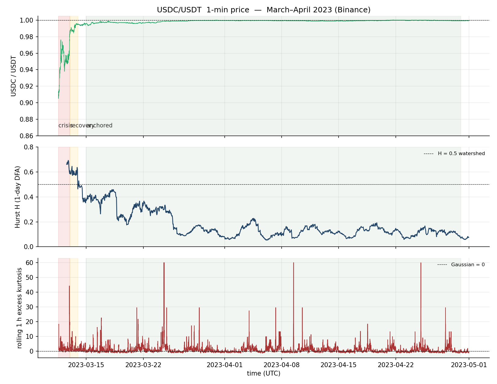
USDC through the SVB event: price, Hurst, and kurtosis
What’s genuinely interesting is the following two phases. In the re-peg, the Hurst median retreats from 0.665 to 0.594; the external intervention signal from the Fed has landed, and the system is no longer drifting toward the critical point, but the old inertia is still there and stays somewhat above ; volatility drops to a third of the crisis level; the tail exponent rebounds to 5.35 and the fat-tailed feature disappears.
By the anchored phase, the Hurst median drops to 0.132, identical to UST’s baseline reading of 0.137; volatility drops another order of magnitude.
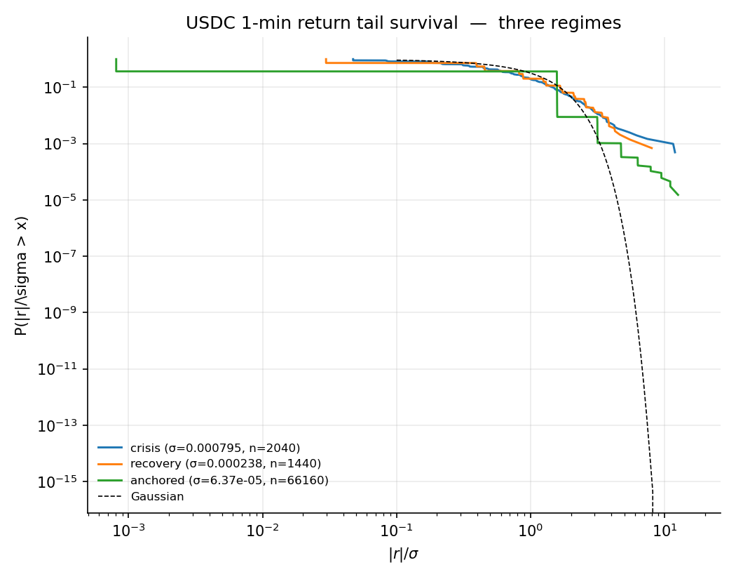
Return-tail survival functions across USDC’s three regimes
The crisis curve (blue) clearly sticks out past the normal reference, walking a near-linear power-law shape; the re-peg curve (orange) is a little thinner but still exceeds normal; the anchored curve (green) returns to a shape that’s within statistical noise of normal.
UST’s case shows what happens when the system crosses the watershed — symmetry breaking and collapse. USDC’s case shows that even when the system only walks up to the watershed without crossing it, the three observables , , and kurtosis still leave a trace that matches the theory perfectly — and once parameters are pulled back to the anchored regime, these traces vanish within tens of hours. The same theory applies equally to the post-collapse recovery: recovery and collapse ought to be highly symmetric, though I haven’t done the math to prove it yet, so I don’t know for sure.
Put both directions together and the message is: before a crisis really arrives, or when one walks up close and brushes past, they both signal the trader in advance — run, fast.